Introduction
“SAS® vs R” has been a hotly debated topic for over a decade. Initially regarded as a tool for academics and enthusiasts, R’s reputation has come a long way. While it was initially used alongside SAS for advanced models and statistical graphics, R’s popularity has surged, leading to increased investment in specialized packages for clinical data programming. This shift has sparked conversations on the synergy between SAS and R, and today, theco industry is increasingly recognizing R as a viable alternative to SAS for various tasks, including SDTM, ADaM, and TFL generation.
What has the transition from being a SAS-only biometric team to a multilingual team actually looked like? Our first step was to take a moment to consider a few key ideas before jumping into the actual transition.
Transition Preparation: Consider Immersion
R, as a language, offers a distinct approach and conceptualization of data compared to SAS. When programmers embark on the journey of learning this new language and strive for fluency, it’s very similar to acquiring a new language in real life. Just like language immersion accelerates learning, immersing ourselves in R has been the fastest and most efficient path to mastery. Expecting programmers to constantly switch between R and SAS during the early stages of the transition can impede fluency and lead to significant frustration. The transition from SAS to R seems to go much more smoothly if programmers are moved to dedicated groups which can focus solely on R for a significant period.
Transition Preparation: Basic R concepts
Just like every programming language, R has its unique characteristics. While SAS boasts a plethora of useful procedures, ranging from the straightforward PROC SORT to the advanced PROC NLMIXED, covering a wide spectrum in between; R, on the other hand, approaches these functionalities in its distinct manner.
R provides out-of-the-box functions within its “base” package, while additional language extensions are housed in various packages. Each package is a collection of R functions designed for specific purposes. Before utilizing them in a program, packages need to be installed and loaded into the R workspace. This packaging system can be loosely compared to a SAS macro library, encompassing multiple functionalities created through specific coding statements and options. The range of packages is vast, spanning from simple string manipulation to comprehensive data visualization.
Unlike SAS, which has procedures created by SAS itself and macros created by users, R embraces a user-centric approach. R users create packages and their corresponding functions, which are then published for open-source use. This user-driven aspect is a strength, placing users at the forefront of innovation. However, it also poses a challenge as the validation of packages may vary. Packages also undergo continuous enhancements, corrections, and adjustments, so it is crucial to carefully review version release notes to assess their impact.
Moving into Fluency: Beyond SAS
As we move beyond the basics, we can begin to get into the meat of what using R looks like. For biometrics teams transitioning from SAS to R, it’s beneficial to draw connections between new R concepts and their similar counterparts in SAS. This helps programmers quickly grasp how to leverage R functions.
For instance, we can use a vector with the “case match” function in R to recode a variable, much like how SAS formats are commonly used. However, it’s crucial to avoid assuming that these concepts function identically behind the scenes. Such misconceptions can limit our progress in R and restrict our flexibility in utilizing R commands. In the given example, SAS formats govern how a variable is displayed, requiring an additional step to modify the raw data values. In contrast, in R, “case match” acts as a vectorized recode function, offering much greater functionality than a simple reformat. It accepts both vectors and single values as input and provides arguments to handle unmatched values.
As we strive for fluency in R, our programming mindset needs to shift from SAS’s line-by-line or row-based approach to R’s column-based process. While this transition may pose some initial challenges, it ultimately enables more flexible and compact programming when approached correctly.
For instance, in SAS, we utilize the “by” statement to process dataset observations in groups. In R, an equivalent commonly found in the dplyr package is the “group by” function. Going beyond this basic equivalence opens up a whole new realm of grouped data processing. Unlike the SAS data step, which is restricted to the current row, grouped data processing in R grants visibility to the entire group. This unlocks exciting possibilities for analyzing and manipulating grouped data.
In R, the fundamental building block is a vector, rather than a single variable. Vectors in R can hold single values but are commonly used as objects, similar to SAS arrays, and can even serve as multi-dimensional arrays. Leveraging vectors in R simplifies tasks like recoding and reformatting. This combination of formatting capabilities and nested array functionality significantly streamlines data manipulation, particularly when transforming large volumes of raw data variables in predictable patterns.
Moving into Fluency: Embracing the Tidyverse
SAS programmers often find comfort in the structured code enclosed between “data” and “run;” or “proc” and “quit;”. In contrast, R exudes a sense of boundless freedom, which can be both liberating and overwhelming. But fear not — there’s a perfect solution to tame this wildness: the Tidyverse! Considered a dialect of the R language, the Tidyverse is a powerful collection of packages that share a common vision, grammar, and data structures.
Within the Tidyverse, data frames take center stage, following a familiar block-based approach like in SAS. Each line connects seamlessly to the next using the pipe operator, “%>%”, which elegantly channels values or data frames forward for further transformations. It’s like a virtual conveyor belt for our data, effortlessly carrying it through the analysis pipeline.
Beginner R programmers who stay within the Tidyverse are likely to feel more secure and confident in their code.
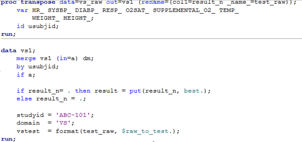
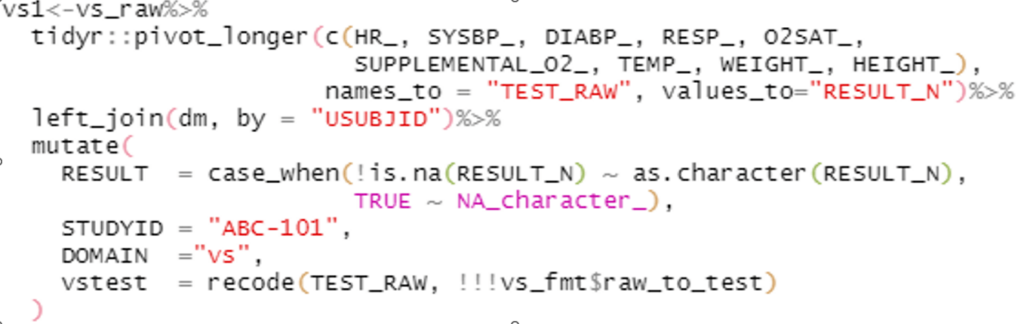
Example 1: Side by side comparison of SAS and tidyverse code for the same task
Moving into Fluency: Utilize available tools
Besides packages and functions, R offers handy tools that can be loaded into the environment to fulfil specific requirements. For instance, unlike SAS which automatically generates a log file, R doesn’t do it by default. However, there’s a nifty tool called “logrx” that comes to the rescue. Once we install it in the RStudio IDE, we can effortlessly generate a log file, saving us from the hassle of manual logging. As each team moves forward and encounters new needs, the key will be finding the right tools to make their R experience even smoother.
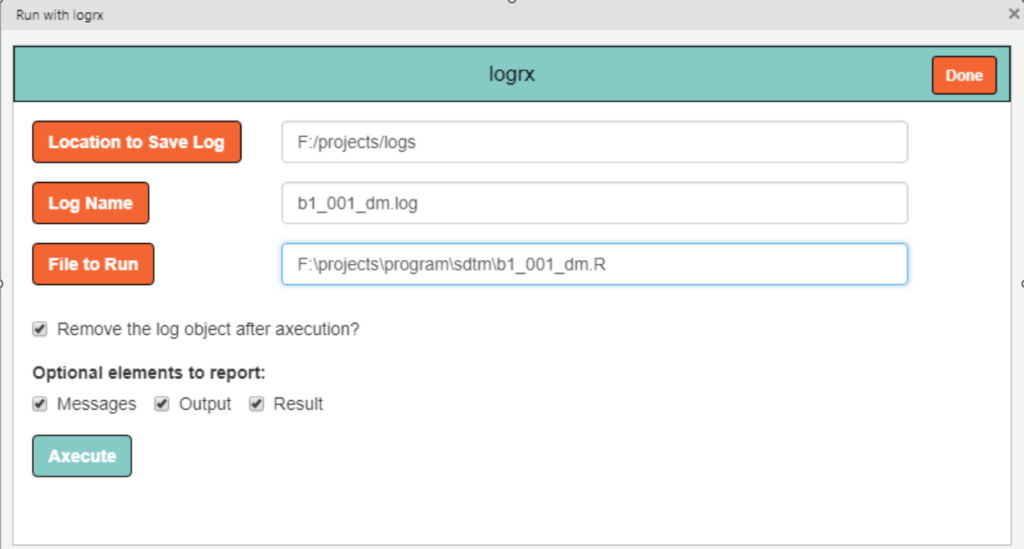
Example 2: User interface of logrx
Moving into Fluency: Under the Hood
As we move into true fluency in R, it is incredibly important to move beyond a surface-level understanding of the functions and packages we are using, to a real knowledge of what is going on under the hood and how these processes differ from what we are used to in SAS. These differences range from very minor and easily solvable to much more complex.
One minor difference is that while SAS sorts null values first in a dataset, R sorts “NA” values last. This difference is fairly easily overcome by replacing all “NA” character values with blanks before sorting or by replacing all NA numeric values with an extremely low, easily identifiable number and all NA dates with something like 1900. These values can then be removed after sorting is complete.
However, there are larger differences. A great example of how SAS and R functions that we might expect to work the same way differ behind the scenes is the rounding function. The SAS round function works the way we learned in basic arithmetic, rounding values ending in 5 to the larger value. For example, 2.5 will round to 3 and 3.5 will round to 4. However, if we think about it, .5 is exactly halfway between the two numbers and there is nothing inherent in a number ending in 5 that would cause it to truly be closer to the higher number. Over time, as we use this approach to rounding, we will end up slowly skewing our data slightly high as we round every .5 to the higher number.
This issue is recognized in computer science, and addressed by the computer science rounding standard, which is to round numbers ending in 5 to the nearest EVEN number. In this case, 2.5 would round to 2 while 3.5 would round to 4. Over large quantities of data, this approach allows for approximately half of the numbers ending in 5 to round down, and half of them to round up, evening out any potential skewing of our data.
This computer science rounding approach is available to us in SAS through the ROUNDE or ROUNDZ functions. It is also the default R rounding function. If we want our R rounding to work the same way as the basic SAS round function, the way we learned to round in elementary arithmetic, we will need something like the R UT_ROUND function, which our team created. This is just one example of how assuming that functions in SAS and R work the same way under the hood can end with unexpected and potentially confusing results.
An even lesser-known difference between the two languages involves how they store numbers in the background. All computing software stores numbers in binary. Usually, converting between binary and decimal isn’t a problem. But here’s the catch: some numbers are rational in decimals but irrational in binary. Take the fraction 1/3, for example. As a fraction, it’s exact and can be added three times to get 1. However, when we convert it to a decimal, we end up with an infinitely repeating number (.33333…). We have to decide where to cut it off, and adding this truncated decimal three times won’t give you exactly 1. So, when we input a number that’s rational in decimals but irrational in binary into our programming language, it has to make decisions on truncation and storage.
Different operating systems handle this slightly differently to maximize the range or precision of stored numbers. Even if we run SAS on two different computers, we might encounter minor discrepancies when working with large amounts of precise data. SAS and R also make slightly different assumptions when it comes to storing these irrational numbers. Usually, it’s not a problem, but occasionally, these small discrepancies can accumulate, making it impossible to perfectly match outcomes after “translating” numbers between decimals, SAS, and R, and rounding them in the end.
Fortunately, it is possible to minimize the effect of these rounding and float point differences by choosing functions which account for these known differences. The tplyr package, for example, utilizes a rounding function that minimizes these discrepancies and matches SAS nearly all of the time.
CDISC Compliance
Fluency in R is an excellent goal, but as biometrics teams, our main purpose is to make sure that we can effectively code to CDISC standards. Fortunately, R has many wonderful packages within the pharmaverse that are specifically designed to assist us in this goal.
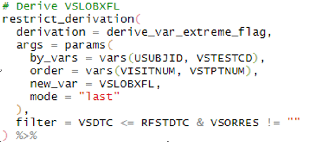
When it comes to programming SDTMs, base R can do the job, some packages make the process much smoother while ensuring CDISC compliance. The dplyr package, for example, is packed with handy functions that let us transform variables in familiar ways, such as using if-then statements or reformatting. In addition, we can filter data, join datasets (à la PROC SQL), and control which columns end up in our final dataset. In addition, the meta tools package is a gem for SDTM work. It helps us check if we have all the required variables, avoid extras, and validate variable values against predefined code lists controlled terminology, and sort datasets by predefined keys. Even the more advanced admiral package can be extremely useful in SDTM programming as it handles the recommended –LOBXFL, calculate reference start and end dates, and much more. These packages are like superpowers for SDTM programming in R!
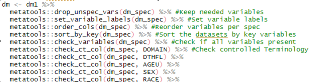
Example 3: dplyr, metatools and admiral in action on SDTM programs
Continuing into ADaM programming, the admiral package truly shines as our go-to tool for deriving almost every variable we need. In addition, the meta tools package is a lifesaver when it comes to manipulating metadata. We can effortlessly read it in, set labels, keep specific variables, and sort them just the way we want for each dataset. To top it off, we have the xportr package. It effortlessly applies formats and dataset labels, making your data presentation a breeze.
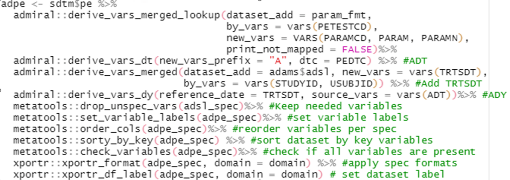
Example 4: meta tools and admiral in action on an ADaM program
As we navigate the world of CDISC standards, it’s crucial to prioritize clear documentation of our metadata and processes. Our programming specifications need to adapt to accommodate the requirements of R programming, which may differ from those of SAS programming due to the unique defaults within packages and procedures.
Furthermore, since R relies heavily on packages that are loaded into the environment, including package information becomes an essential part of our documentation strategy. We should consider incorporating this information into the ADRG (Analysis Data Reviewer’s Guide) and the cSDRG (Define-XML SDRG).
In the ADRG, Section 7, aptly titled “Submission of Programs,” we can dedicate a space to include package details. This way, we ensure that the reviewers and stakeholders have a comprehensive understanding of the tools and packages utilized in our analysis. In the cSDRG, we can integrate this information within domain-specific sections or include it as an appendix for easy reference.
By proactively documenting the usage of packages and their impact on our analyses, we enhance transparency and provide valuable insights into our R programming approach.
During the Transition: Ensuring Quality
Once we are aware of what this transition from SAS to multilingual might entail, there are a few practices that can help us navigate the transition smoothly, ensuring the quality and consistency of our work throughout the process.
First and foremost, we have found independent programming to be highly effective. By dedicating one side to SAS for production and the other to R for quality control (QC), or vice versa, we gain a clear view of any discrepancies between the two languages. This allows us to address and resolve any differences confidently.
To establish a solid foundation, it can also be beneficial to match existing SAS QC’d results using R. When a dataset or table has already undergone QC in SAS, the programmer can focus on achieving matching results in R. This approach reduces the chances of discrepancies arising from mistakes in the production SAS code, enabling us to concentrate on finding effective methods for replicating the results in R.
Throughout the transition, we may discover additional details and requirements specific to R that were previously assumed or not needed in SAS. To ensure a smooth shift towards using R on both sides of the process, it is crucial to identify these extra details and incorporate them into the necessary documentation, such as SAP, specifications, and reviewer’s guides. By doing so, we can avoid overlooking essential information or making different assumptions when SAS is no longer employed as a double-check. Since R provides more flexibility for customization compared to SAS, comprehensive and detailed documentation becomes even more crucial to establish clear project assumptions.
Lastly, while we often stress the importance of detailed comments in SAS programming, it is equally essential to encourage programmers to embrace this practice in their R programs. During the learning process, it’s easy to become engrossed in solving problems or completing datasets in R. However, thorough commenting can save valuable time and effort by avoiding the need to solve the same problem from scratch in the future. This becomes even more crucial when team members are learning and transitioning, as detailed comments not only benefit the programmer themselves but also facilitate improvement through review and feedback from more experienced programmers.
By implementing these practices, we can confidently navigate the transition, ensuring high-quality work, maintaining consistency, and fostering effective collaboration within the team.
Into the Future
Hopefully, at this point, it is clear that the transition from a team that only uses SAS to a team that can use either SAS or R to meet the same goals is completely possible. However, the truly exciting things about R lie in its possibilities and potential as we move into the future of our industry.
R opens up exciting possibilities, enabling us to embrace the advancements in technology-driven reviews that are prevalent today. Gone are the days of printing out stacks of paper to review an entire study. With the power of technology at our fingertips, why should we settle for static tables and figures? Enter RShiny, a fantastic tool that revolutionizes data exploration by creating interactive tables and figures.
With RShiny, users can dive deep into the data points through interactive features. Imagine selecting specific points on a data visualization or plot, and instantly generating a table or listing that exclusively displays those selected points. Furthermore, hovering over a single line in a line plot can highlight specific groups, offering a detailed view of subject-level values and summary statistics. The flexibility is incredible!
In just a click, users can sort, filter, and perform various operations on tables, figures, and listings, eliminating the need to write code for individual outputs in each situation. In a static environment, exploring data at a high level would require generating separate tables or plots for each group. While static outputs still have their place in publications and clinical study reports, the advantages of this level of dynamic data investigation for experimental therapies are immense.
RShiny empowers us to unleash the full potential of our data, facilitating in-depth analysis, enhanced exploration, and an interactive user experience. It’s a game-changer that propels us into the future of technology-driven reviews.

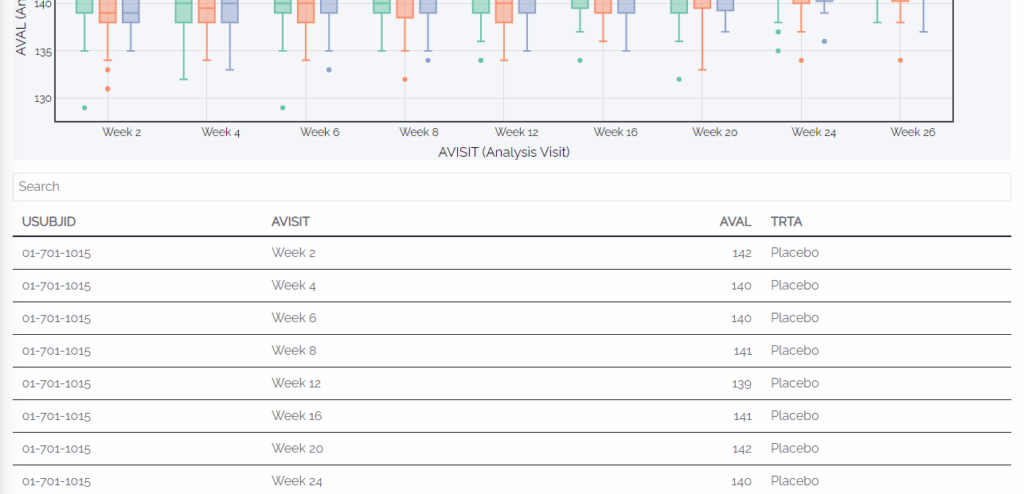
Example 5: RShiny box plot with the visit and PARAMCD filters in place and summary stats showing when hovered over, plus an automatically filtered data listing associated with the box plot.
To Wrap It Up
Not everyone is a language aficionado. In fact, many programmers in our industry did not come into it with a computer science degree and have never had to learn multiple programming languages. While exciting and adventurous to some, others can find the mere suggestion of an industry diving into a new programming language to be daunting at best. However, the beauty of this transition is that we don’t have to start from scratch.
Numerous resources are available to support SAS programmers as they venture into the realm of R. By following the guidance and insights of those who have already embarked on this journey, and by asking plenty of questions along the way, you’ll discover that R offers a more powerful, customizable, and user-friendly toolset than SAS has proven to be. By keeping an open mind and continually exploring the capabilities of R, before you know it, you’ll become proficient in multiple programming languages, opening up a world of possibilities.
So, let’s embrace the adventure, leverage the knowledge of others, and dive into the world of R. With persistence and curiosity, you’ll soon find yourself fluent in this new language, ready to unlock new insights and drive innovation in our industry. The journey may seem daunting, but remember that you’re not alone, and the rewards of mastering R are well worth the effort. Happy programming!