
So – it’s been longer than a week… I wasn’t born to be a blogger, but that’s ok.
If you’re new to this blog series, head on over to part 1 to catch up on what we’re doing here. That first post sets the stage, gives motivation to the problem, and sets the parameters of the challenge. For the latest in this series, go and check out post 3.
Let’s take a look at the next attempt.
Solution 3: Better use of {stringr}
#' @param text String to be wrapped
#' @param width Longest allowable width of a line
#'
#' @return Wrapped string
overflow_wrap3 <- function(text, width) {

   # Find where the splits need to happen
   sections <- str_locate_all(text, paste0("\\w{", width-1, "}(?=\\w)"))[[1]]

   # Using the locations, build up the matrix of substrings
   split_mat <- matrix(c(1, sections[,2]+1, sections[,2], -1), ncol=2)

   # Dive the string into the necessary chunks
   splits <- str_sub(text, split_mat)

   hyph_str <- paste(splits, collapse = "- ")

   # Wrap the final string
   str_wrap(hyph_str, width)
}

# Vectorization of overflow_wrap3
overflow_wrapper3 <- Vectorize(overflow_wrap3, vectorize.args = "text")
This is quite a bit cleaner, isn’t it? Compared to the last post, no more in place modifying or playing with the namespaces. Here, we do things more sequentially.
- We find the locations of hyphens we need to insert
- Build a matrix of substrings to segment our strings into proper pieces
- Join everything back together with the necessary segments split by hyphenationm, and finally
- Wrap all of the lines using good ol’
stringr::str_wrap()
With less messing around, and more leveraging of proper ways that stringr was written, we trim some more time off the clock.
With this approach, one thing we can certainly do is start trying to use {stringr} in the way it was intended. At first, it feels kind of funky that stringr::str_locate_all() returns list of matrices. That’s not a data type you might be used to seeing, particularly when working with basic string operations. Sure, the matrix structure is a good representation of the data being returned here, but at first it felt a bit odd to work with compared to other tidyverse functions. That is, until you realize that the output of stringr::str_locate_all() can be fed directly into stringr::str_sub().
x <- c("This is the best blog post I've ever read.")

locs <- stringr::str_locate_all(x, r"(blog|ever)") # This is using a raw string, new in R 4.0

stringr::str_sub(x, locs[[1]])
[1] "blog" "ever"
So let’s play that out. To simplify the example, here I’m just searching for the words “blog” or “ever”. Sticking with our original motivation, the trick here becomes that I don’t want the locations of the individual words – I want the chunks of this string split at the points where I want to insert the hyphen. So instead I want to separate my string into this:
"This is the best blog" " post I've ever" " read." Let’s take a look at the actual data. The below matrix is what’s initially returned to us by stringr::str_locate_all(), inside the locs variable.
 start end
    18  21
    33  36
If you dig into the string, you’ll se that the location of “blog” is character 18 through 21, and the location of “ever” is character 33 through 36. So now what do we want this to look like?
 start end
     1  21
    22  36
    37  -1
Note that labels to the columns have been added for clarity
Notice the pattern – I’m going from the beginning to the end of the string (signified by -1). At the end of each match, I hit an end point, and the start point of the next row is the previous endpoint + 1. Once you wrap your head around the desired pattern (which may take a minute – it did for me), creating this matrix is quite concise.
split_mat <- matrix(c(1, m[,2]+1, m[,2], -1), ncol=2)
split_mat
     [,1] [,2]
[1,]    1   21
[2,]   22   36
[3,]   37   -1
While this is concise, it admittedly looks confusing – so let’s go through it.
- The starting point here is matrix
mwhich I pulled from thelocsobject returned bystring::str_locate_all(). Let’s take another look at what this looks like
locs[[1]]
     start end
[1,]    18  21
[2,]    33  36
Now things get a little weird.
- To start with the easy part, we want ‘start’ on the first row to be 1, and we want ‘end’ on the last row to be -1. This symbolizes the start and end of the entire string of interest.
- Next, we want all of the start points to be the character directly after the end points identified by our original search from
stringr::str_locate_all(). This was an important part for us to edit, because we want the string chunking to just pick up right after the last chunk ends instead of waiting until our next identified word starts. We add this by pulling the “end” column and adding 1 asm[,2]+1. - Last, we want all of the originally identified end points. So we pull this just as
m[,2]. - To fit it all together, we tie it all in as one vector, which looks like this:
c(1, m[,2]+1, m[,2], -1)
 1 22 37 21 36 -1
We’re getting there, but it’s not quite what we want yet.
- We need to convert it back into a matrix. The way we built this, the first half we want as the ‘start’ column and the last half as the ‘end’. So we use the
matrix()function for this:
matrix(c(1, m[,2]+1, m[,2], -1), ncol=2)
     [,1] [,2]
[1,]    1   21
[2,]   22   36
[3,]   37   -1
And there we go! It was a complicated step, but the result is simply that you have a matrix outlining each individual chunk of the string. Popping it into stringr::str_sub() we get this beauty.
str_sub(x, matrix(c(1, locs[[1]][,2]+1, locs[[1]][,2], -1), ncol=2))
[1] "This is the best blog" " post I've ever"       " read."
How cool is that! In three lines we’re already at the point where we just need to collapse this character vector back together. So it’s a simple paste(), and then we’re off to the races with stringr::str_wrap().
So most the overhead should be gone now, right?
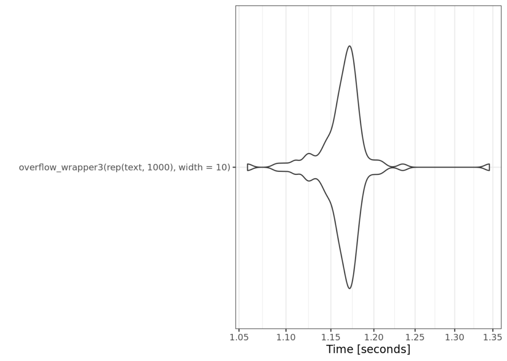
Admittedly this wasn’t what I expected. We only cut off .2 seconds from the last example. So this brings up an interesting question of where exactly this overhead is coming from. I spent some time in RStudio’s profiler, but struggled to understand exactly where the extra 1.12 seconds is coming from. Take a look at the code, and ruminate on this. Where do you thinking the inefficiency could be coming from? Where are we potentially doing extra work?
In my next post, we’ll get some answers. Because the next post is the last in this series! So keep your eyes peeled. I won’t say next week, but the last post will be out soon!
As a reminder – you can submit your solutions in our GitHub repo, which has submission instructions in the README.